Chapter 4 · Matrix Decompositions
End-of-chapter exercises. Each has a definitions box, explanation, worked steps, and the answer.
4.1 · Determinant via Laplace and Sarrus
Compute the determinant of
using the Laplace expansion (along the first row) and Sarrus' rule.
Topics & Definitions
- Laplace expansion — pick any row or column; for each entry delete its row and column to form the minor, take that minor's determinant, multiply by the entry, attach a checkerboard sign, and sum: \(\det(A) = \sum_{k=1}^{n} (-1)^{j+k}\, a_{jk}\, \det(A_{j,k})\).
- Checkerboard signs — for a \(3\times3\) they are \(\begin{pmatrix}+&-&+\\-&+&-\\+&-&+\end{pmatrix}\). A zero entry contributes a zero term, so its minor never needs computing. Expand along the row or column with the most zeros; every line gives the same answer, so pick the laziest one.
- Sarrus' rule — a \(3\times3\)-only shortcut: copy the first two columns to the right, add the three down-right (\(\searrow\)) diagonal products, and subtract the three up-right (\(\nearrow\)) ones. Does not generalise beyond \(3\times3\).
- Zero determinant — the columns are linearly dependent, the parallelepiped they span is squashed flat (zero volume), and \(A\) is not invertible (singular).
Both methods must land on the same number, so computing it two ways is a built-in cross-check. Laplace along row 1 uses the signs \(+, -, +\); Sarrus reads six diagonal products.
Method 1, Laplace along the first row
Row 1 is \((1, 3, 5)\) with signs \(+, -, +\) from the checkerboard.
Entry \(a_{11} = 1\), sign \(+\). Delete row 1 and column 1:
Entry \(a_{12} = 3\), sign \(-\). Delete row 1 and column 2:
Entry \(a_{13} = 5\), sign \(+\). Delete row 1 and column 3:
Assemble:
Common slip
The alternating \(+, -, +\) on the first row is where most sign errors happen. Dropping the minus on the middle term would give \(4 + 24 + 20 = 48\) instead of \(0\).
Method 2, Sarrus' rule
Copy the first two columns to the right:
Down-right diagonals (\(\searrow\)), added:
Up-right diagonals (\(\nearrow\)), subtracted:
Answer
Both methods agree, a useful cross-check whenever two independent routes are available. A zero determinant means \(A\) is singular: its columns are linearly dependent, the parallelepiped they span has collapsed to zero volume, and \(A^{-1}\) does not exist. This exercise is quietly a "spot the singular matrix" question, not just an arithmetic drill.
4.2 · Computing a \(5\times5\) determinant efficiently
Compute the determinant of
efficiently.
Topics & Definitions
- "Efficiently" is the whole exercise — a naive Laplace expansion of a \(5\times5\) spawns five \(4\times4\) minors, each spawning four \(3\times3\)s, that is \(20\) sub-determinants. Done well, this needs the real computation of just one \(4\times4\).
- Expand along the most zeros — every zero entry gives a zero term, so its minor never needs building. Any row or column gives the same answer, so pick the laziest one.
- Identical rows or columns force \(\det = 0\) — they are linearly dependent, so the spanned parallelepiped collapses to zero volume. Skip the expansion entirely. A row or column of all zeros does the same.
- Track signs as three factors — when the entry multiplying a minor is itself negative, the double negative is an easy place to lose a sign. Keep \((\text{sign}) \times (\text{entry}) \times (\text{minor})\) as three separate pieces.
Before expanding anything, look at the matrix. Find the line with the most zeros to expand along, and watch for duplicate rows or columns that zero a minor for free. Here both tricks apply, so almost no arithmetic is needed.
Step 1, count the zeros
| Column | Entries | Zeros |
|---|---|---|
| 1 | \(2, 2, 0, -2, 2\) | 1 |
| 2 | \(0, -1, 1, 0, 0\) | 3 ⭐ |
| 3 | \(1, 0, 2, 2, 0\) | 2 |
| 4 | \(2, 1, 1, -1, 1\) | 0 |
| 5 | \(0, 1, 2, 2, 1\) | 1 |
Column 2 wins. Only two of its five entries are nonzero: \(-1\) at row 2 and \(1\) at row 3. Three terms die immediately, leaving just two \(4\times4\) minors instead of five.
Step 2, the two surviving minors
Entry \(a_{22} = -1\), sign \((-1)^{2+2} = +1\). Delete row 2 and column 2:
Entry \(a_{32} = 1\), sign \((-1)^{3+2} = -1\). Delete row 3 and column 2:
Free win, do not expand this one
Rows 2 and 4 of \(M_2\) are identical (\(2, 0, 1, 1\) both times). Identical rows force \(\det(M_2) = 0\) with no computation at all. Spotting this saves an entire \(4\times4\) expansion.
Step 3, assemble
Note the first term: the entry is \(-1\) and the minor is \(-6\), so the two negatives cancel to give \(+6\).
Answer
What made it efficient. The naive route is \(20\) sub-determinants. Here column 2's three zeros cut five minors down to two, \(M_2\)'s duplicate rows made it zero for free, and only one \(4\times4\) ever needed real work. The exercise tests strategy, not arithmetic: scan for zeros and duplicate lines before computing anything, the single highest-leverage move in the whole determinants topic.
4.3 · Computing eigenspaces
Compute the eigenspaces of
Topics & Definitions
- Eigenvalue equation — \(\lambda\) is an eigenvalue of \(A\) if \(Av = \lambda v\) for some nonzero \(v\). Rearranged, \((A - \lambda I)v = 0\), which needs \(A - \lambda I\) singular, so \(\det(A - \lambda I) = 0\). That is the characteristic polynomial, and its roots are exactly the eigenvalues.
- Workflow — form \(A - \lambda I\) (subtract \(\lambda\) down the diagonal), compute its determinant, set it to zero and solve for the eigenvalues, then for each \(\lambda\) separately solve \((A - \lambda I)v = 0\) for its eigenspace. Each eigenvalue gets its own system and its own answer; they are never combined.
- Free variables are the point — when solving \((A - \lambda I)v = 0\) the rows always go redundant (that is exactly why \(\lambda\) was chosen), so a row reducing to \(0 = 0\) constrains nothing and gets crossed out. The unconstrained variable spans the eigenspace. Careful: \(0v_1 + 0v_2 = 0\) says nothing about \(v_2\); multiplying by zero destroys the information, so it cannot "see" the variable at all.
- Scaling is free — \((1,3)\), \((2,6)\), and \((-1,-3)\) all span the same line, so pick the cleanest integer representative.
- Two multiplicities — the algebraic multiplicity is how many times \(\lambda\) is a root; the geometric multiplicity is the dimension of its eigenspace. They need not match, and you have to solve the system to find out.
The recipe is the same for both matrices: build the characteristic polynomial, find its roots, then solve a separate singular system for each root. Part a lands on one repeated eigenvalue; part b on two distinct ones.
Part a, characteristic polynomial
Setting to zero, \((\lambda - 1)^2 = 0 \Rightarrow \lambda = 1\): a single eigenvalue, but a repeated root, so algebraic multiplicity \(2\).
Part a, eigenspace for \(\lambda = 1\)
Substitute \(\lambda = 1\):
Reading \((A - I)v = 0\) row by row: row 1 is \(0v_1 + 0v_2 = 0\), no information, discard; row 2 is \(v_1 = 0\). So \(v_1 = 0\) and \(v_2\) is free:
Check: \(A\begin{pmatrix}0\\1\end{pmatrix} = \begin{pmatrix}0\\1\end{pmatrix} = 1\cdot\begin{pmatrix}0\\1\end{pmatrix}\). \(\checkmark\)
Part b, characteristic polynomial
Factorising (two numbers multiplying to \(-6\) and summing to \(+1\), namely \(-2\) and \(3\)):
Two distinct eigenvalues, so two separate eigenspaces.
Part b, eigenspace for \(\lambda = 2\)
Row 1: \(-4v_1 + 2v_2 = 0 \Rightarrow v_2 = 2v_1\). Row 2: \(2v_1 - v_2 = 0 \Rightarrow v_2 = 2v_1\) (the same information, as expected). Taking \(v_1 = 1\):
Check: \(B\begin{pmatrix}1\\2\end{pmatrix} = \begin{pmatrix}2\\4\end{pmatrix} = 2\begin{pmatrix}1\\2\end{pmatrix}\). \(\checkmark\)
Part b, eigenspace for \(\lambda = -3\)
Row 1: \(v_1 + 2v_2 = 0 \Rightarrow v_1 = -2v_2\). Row 2: \(2v_1 + 4v_2 = 0 \Rightarrow v_1 = -2v_2\) (redundant, as expected). Taking \(v_2 = 1\):
Check: \(B\begin{pmatrix}-2\\1\end{pmatrix} = \begin{pmatrix}6\\-3\end{pmatrix} = -3\begin{pmatrix}-2\\1\end{pmatrix}\). \(\checkmark\)
Answer
a) One eigenvalue \(\lambda = 1\), with a one-dimensional eigenspace:
b) Two eigenvalues, each with a one-dimensional eigenspace:
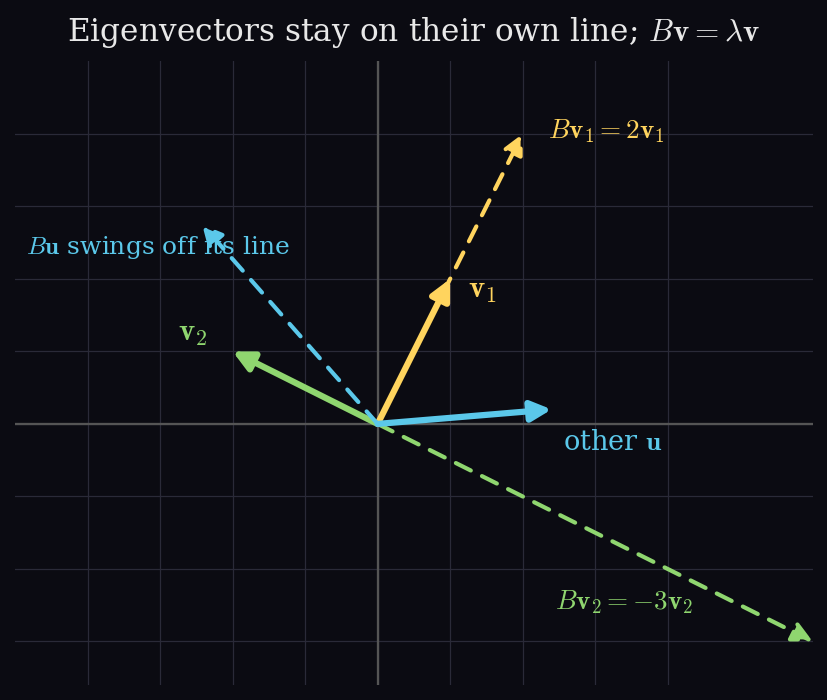
Part a is defective. The eigenvalue \(\lambda = 1\) has algebraic multiplicity \(2\) but geometric multiplicity \(1\): a \(2\times2\) matrix yielding only one independent eigenvector direction. Geometrically \(A\) is a shear, leaving the \(y\)-axis fixed but tilting everything else, so only one line survives unchanged. Such a matrix is not diagonalisable.
Part b's eigenvectors are orthogonal. \((1,2)\cdot(-2,1) = -2 + 2 = 0\). This is not luck: \(B\) is symmetric, and symmetric matrices always have orthogonal eigenvectors for distinct eigenvalues.
4.4 · Eigenspaces of a \(4\times4\) (a defective matrix)
Compute all eigenspaces of
Topics & Definitions
- Same method, just bigger — form \(A - \lambda I\) and compute \(\det(A - \lambda I)\) (the characteristic polynomial), factorise and set to zero for the eigenvalues, then for each eigenvalue solve \((A - \lambda I)v = 0\) by row reduction for its eigenspace.
- Two free sanity checks — before factorising, verify the coefficient of \(\lambda^{n-1}\) equals \(-\operatorname{tr}(A)\) and the constant term equals \(\det(A)\). Here \(\operatorname{tr}(A) = 1\) and \(\det(A) = 2\), so the \(\lambda^3\) coefficient must be \(-1\) and the constant must be \(2\). A mismatch means a slip upstream, catch it before wasting effort factorising.
- Reading an eigenspace off an RREF — a column with a leading \(1\) is a pivot, so that variable is pinned; a column with no leading \(1\) is free and spans the eigenspace. A non-leading entry (a stray \(-1\), say) does not make a column a pivot.
- Algebraic vs geometric multiplicity — algebraic is how many times \(\lambda\) is a root; geometric is the dimension of the eigenspace, i.e. the number of free variables. When geometric \(<\) algebraic the matrix is defective and cannot be diagonalised.
The size jumps to \(4\times4\) but nothing conceptual changes. The one thing to watch is the repeated root: an eigenvalue can appear twice in the polynomial yet still hand back only a single eigenvector direction.
Step 1, characteristic polynomial
Expanding \(\det(A - \lambda I)\) by Laplace along column 4 (its zero entry kills one term, leaving three minors):
Check: the \(\lambda^3\) coefficient is \(-1 = -\operatorname{tr}(A)\) \(\checkmark\), and the constant is \(2 = \det(A)\) \(\checkmark\).
Step 2, factorise
By the rational root test the candidates are \(\pm1, \pm2\). Testing \(\lambda = 1\) gives zero, so \((\lambda - 1)\) is a factor; dividing out and repeating:
Eigenvalues: \(\lambda = -1\) (algebraic multiplicity \(2\)), \(\lambda = 1\), \(\lambda = 2\). Multiplicities sum to \(4\) \(\checkmark\).
Step 3, eigenspace for \(\lambda = 2\)
Row-reduce \(A - 2I\); one free variable remains, giving
Check: \(A(1,0,1,1)^\top = (2,0,2,2)^\top = 2(1,0,1,1)^\top\). \(\checkmark\)
Step 4, eigenspace for \(\lambda = 1\)
Row-reduce \(A - I\); one free variable:
Check: \(A(1,1,1,1)^\top = (1,1,1,1)^\top = 1\cdot(1,1,1,1)^\top\). \(\checkmark\)
Step 5, eigenspace for \(\lambda = -1\)
Row-reduce \(A + I\). The RREF is
Pivots sit in columns 1, 2, 4, so only column 3 is free, a single free variable. Reading the rows: \(v_1 = 0\), \(v_2 = v_3\), \(v_4 = 0\). Hence
Check: \(A(0,1,1,0)^\top = (0,-1,-1,0)^\top = -1\cdot(0,1,1,0)^\top\). \(\checkmark\) Despite \(\lambda = -1\) having algebraic multiplicity \(2\), its eigenspace is only \(1\)-dimensional.
Answer
This matrix is defective. The eigenvalue \(\lambda = -1\) has algebraic multiplicity \(2\) but geometric multiplicity \(1\). The geometric multiplicities sum to \(1 + 1 + 1 = 3\), short of the matrix size \(4\), so there are not enough independent eigenvectors to form a basis: \(A\) is not diagonalisable.
4.5 · Diagonalizability vs invertibility
Diagonalizability of a matrix is unrelated to its invertibility. Determine for the following four matrices whether they are diagonalizable and/or invertible:
Topics & Definitions
- The point — diagonalizability and invertibility are independent. A matrix can have either, both, or neither, because they are checked by completely different criteria.
- Invertible — asks whether the map loses information: invertible \(\iff \det(A) \neq 0 \iff\) no eigenvalue equals \(0\). A zero eigenvalue crushes a direction to nothing, which cannot be undone.
- Diagonalizable — asks whether there are enough independent eigenvectors to span the space, i.e. for every eigenvalue the geometric multiplicity equals the algebraic multiplicity. When they fall short, the matrix is defective and not diagonalizable.
- Why they are unrelated — invertibility asks "is any eigenvalue zero?"; diagonalizability asks "are there enough eigenvectors?". Different questions, so all four yes/no combinations can occur, which is exactly what these matrices show.
Triangular shortcut
For a triangular matrix the eigenvalues are just the diagonal entries. All four matrices here are triangular, so their eigenvalues can be read straight off.
Matrix 1, the identity
Eigenvalues \(1, 1\) (from the diagonal). Neither is zero, so \(\det = 1 \neq 0\): invertible. Every vector satisfies \(Iv = v\), so the whole plane is the eigenspace for \(\lambda = 1\): geometric multiplicity \(2\) matches algebraic multiplicity \(2\), so diagonalizable (it is already diagonal).
Matrix 2, a projection
Eigenvalues \(1, 0\). One eigenvalue is zero, so \(\det = 0\): not invertible. Two distinct eigenvalues in a \(2\times2\) always give two independent eigenvectors (here \((1,0)\) and \((0,1)\)), which span the space, so diagonalizable (already diagonal).
Matrix 3, a shear
Eigenvalues \(1, 1\). Neither is zero, so \(\det = 1 \neq 0\): invertible. Solving \((A - I)v = 0\) gives only the single direction \((1,0)\): algebraic multiplicity \(2\) but geometric multiplicity \(1\). Not enough eigenvectors, so not diagonalizable (defective).
Matrix 4, a nilpotent shear
Eigenvalues \(0, 0\). Zero is an eigenvalue, so \(\det = 0\): not invertible. Solving \((A - 0I)v = 0\) gives only \((1,0)\): algebraic multiplicity \(2\) but geometric multiplicity \(1\), so not diagonalizable (defective).
Answer
| Matrix | Invertible | Diagonalizable |
|---|---|---|
| \(\begin{pmatrix}1&0\\0&1\end{pmatrix}\) | Yes | Yes |
| \(\begin{pmatrix}1&0\\0&0\end{pmatrix}\) | No | Yes |
| \(\begin{pmatrix}1&1\\0&1\end{pmatrix}\) | Yes | No |
| \(\begin{pmatrix}0&1\\0&0\end{pmatrix}\) | No | No |
All four combinations appear, confirming the two properties are completely independent: invertibility depends on whether any eigenvalue is zero, diagonalizability on whether there are enough independent eigenvectors.
4.6 · Eigenspaces and diagonalizability
Compute the eigenspaces of the following transformation matrices and decide whether they are diagonalizable.
Topics & Definitions
- Diagonalizability test — an \(n \times n\) matrix is diagonalizable if and only if it has \(n\) linearly independent eigenvectors, enough to form a basis.
- The multiplicity condition — equivalently, for every eigenvalue the geometric multiplicity (dimension of its eigenspace) must equal its algebraic multiplicity (how many times it is a root). A single mismatch makes the whole matrix not diagonalizable (defective).
- Symmetry is a red herring — symmetric matrices are always diagonalizable, but the converse is false: plenty of non-symmetric matrices diagonalize fine. So \(A^\top \neq A\) tells you nothing; the deciding factor is always the eigenvector count.
- A zero eigenvalue is fine — \(\det(A - \lambda I) = 0\) is exactly the condition that makes \(\lambda\) an eigenvalue. If that happens at \(\lambda = 0\) (a vanishing constant term), zero is simply an eigenvalue: the matrix is singular but may still diagonalize.
- Quick check — add up the geometric multiplicities. If they sum to \(n\), the matrix is diagonalizable; if they fall short, it is not.
Part a
Find the eigenvalues, compute each eigenspace, then tally the geometric multiplicities. The repeated eigenvalue is where the surprise lives: it can be a double root yet contribute only a single eigenvector direction.
Step 1, characteristic polynomial
Expanding \(\det(A - \lambda I)\):
Eigenvalues: \(\lambda = 5\) (algebraic multiplicity \(1\)) and \(\lambda = 1\) (algebraic multiplicity \(2\)). Sanity check: sum of eigenvalues \(5 + 1 + 1 = 7 = \operatorname{tr}(A)\) \(\checkmark\), product \(5\cdot1\cdot1 = 5 = \det(A)\) \(\checkmark\).
Step 2, eigenspace for \(\lambda = 5\)
Row-reduce \(A - 5I\); one free variable gives
Geometric multiplicity \(1\), matching its algebraic multiplicity.
Step 3, eigenspace for \(\lambda = 1\)
Row-reduce \(A - I\). Despite \(\lambda = 1\) being a repeated root, only one free variable remains:
Geometric multiplicity \(1\), but algebraic multiplicity \(2\): a mismatch.
Step 4, diagonalizable?
Count the independent eigenvectors:
A \(3\times3\) matrix needs \(3\) independent eigenvectors to be diagonalizable. Only \(2\) exist, so \(A\) is not diagonalizable. The shortfall is at \(\lambda = 1\), whose eigenspace is one dimension smaller than its algebraic multiplicity.
Answer
Not diagonalizable. The eigenvalue \(\lambda = 1\) has algebraic multiplicity \(2\) but geometric multiplicity \(1\), so \(A\) has only \(2\) independent eigenvectors, one short of the \(3\) needed for a \(3\times3\). The matrix is defective.
Part b
Three all-zero rows make \(A\) singular, so \(\det(A) = 0\) and zero will be an eigenvalue. The interesting question is whether its eigenspace is big enough to make up the full multiplicity.
Step 1, characteristic polynomial
Only the top-left entry \(1-\lambda\) survives the expansion, times a diagonal minor:
A vanishing constant term is a signal, not an error
When \(\det(A - \lambda I)\) has no constant term, it means \(\lambda = 0\) is a root, i.e. zero is an eigenvalue. That is different from "there are no eigenvalues." A zero eigenvalue is perfectly valid; it means the matrix crushes some direction to nothing, consistent with \(\det(A) = 0\) (not invertible).
Step 2, solve
Factorise \(\lambda^3(1 - \lambda) = 0\): the factor \(\lambda^3\) gives \(\lambda = 0\) and \(1 - \lambda = 0\) gives \(\lambda = 1\). Eigenvalues: \(\lambda = 0\) (algebraic multiplicity \(3\), from \(\lambda^3\)) and \(\lambda = 1\) (algebraic multiplicity \(1\)). Four roots total, matching the \(4\times4\) size.
Step 3, eigenspace for \(\lambda = 0\)
Solve \(Av = 0\) (the null space of \(A\)). Only the first row constrains anything (\(v_1 + v_2 = 0\)), leaving three free variables:
Geometric multiplicity \(3\), matching the algebraic multiplicity.
Step 4, eigenspace for \(\lambda = 1\)
Solve \((A - I)v = 0\); one free variable:
Answer
Diagonalizable. The eigenvectors number \(3 + 1 = 4\), enough for a \(4\times4\), and both eigenvalues have geometric multiplicity equal to algebraic multiplicity. So \(A\) is diagonalizable even though it is singular: diagonalizability and invertibility are independent, and this matrix has a zero eigenvalue yet still diagonalizes.
4.7 · Diagonal form and eigenbasis
Are the following matrices diagonalizable? If yes, determine their diagonal form and a basis with respect to which the transformation matrix is diagonal. If no, give reasons.
Topics & Definitions
- Diagonalization — \(A\) is diagonalizable if there is a basis of eigenvectors. In that basis \(A\) becomes a diagonal matrix \(D\) of eigenvalues, and \(A = PDP^{-1}\) where the columns of \(P\) are the eigenvectors, ordered to match the eigenvalues in \(D\). The eigenbasis is exactly those columns.
- The test — an \(n \times n\) matrix is diagonalizable iff it has \(n\) linearly independent eigenvectors, equivalently every eigenvalue's geometric multiplicity equals its algebraic multiplicity.
- Real vs complex — the characteristic polynomial may have no real roots. Over the reals such a matrix is not diagonalizable (no real eigenbasis). A negative discriminant is the signal, since it forces complex eigenvalues.
- Discriminant check for a \(2\times2\) — for \(\lambda^2 + b\lambda + c\) the roots are real only if \(b^2 - 4c \geq 0\). If it is negative, the eigenvalues are complex and the matrix is not diagonalizable over \(\mathbb{R}\).
Part a
Part a, characteristic polynomial
Using the \(2\times2\) form \(\lambda^2 - \operatorname{tr}(A)\lambda + \det(A)\), with \(\operatorname{tr}(A) = 4\) and \(\det(A) = (0)(4) - (1)(-8) = 8\):
Part a, solve
The discriminant is \((-4)^2 - 4(8) = 16 - 32 = -16 < 0\). Applying the quadratic formula:
The eigenvalues are complex (\(2 + 2i\) and \(2 - 2i\)).
Answer
Not diagonalizable over \(\mathbb{R}\). The characteristic polynomial \(\lambda^2 - 4\lambda + 8\) has no real roots, its eigenvalues \(2 \pm 2i\) are complex, so there is no real eigenbasis and no real diagonal form. (Over \(\mathbb{C}\) it is diagonalizable, since the two complex eigenvalues are distinct, but with respect to a real basis it is not.)
Part b
Part b, characteristic polynomial
Expanding \(\det(A - \lambda I)\) for the all-ones matrix:
Check: \(\operatorname{tr}(A) = 3\) matches the eigenvalue sum \(0 + 0 + 3\) \(\checkmark\), and \(\det(A) = 0\) matches the product \(\checkmark\). Eigenvalues: \(\lambda = 0\) (algebraic multiplicity \(2\)) and \(\lambda = 3\) (algebraic multiplicity \(1\)).
Part b, eigenspace for \(\lambda = 0\)
Solve \(Av = 0\). Every row of \(A\) is identical (\(v_1 + v_2 + v_3 = 0\)), leaving two free variables:
Geometric multiplicity \(2\), matching the algebraic multiplicity.
Part b, eigenspace for \(\lambda = 3\)
Solve \((A - 3I)v = 0\); one free variable:
Answer
Diagonalizable. The eigenvectors number \(2 + 1 = 3\), enough for a \(3\times3\), and every eigenvalue's geometric multiplicity equals its algebraic multiplicity.
Diagonal form:
Eigenbasis (columns of \(P\), ordered to match \(D\)):
With respect to this basis the transformation is diagonal with entries \(0, 0, 3\).
Part c
Topics & Definitions
- Only repeated eigenvalues can break diagonalizability — an eigenvalue with algebraic multiplicity \(1\) always has geometric multiplicity \(1\), so it can never mismatch. When the question is just "diagonalizable, and if not why," find the eigenvalues, then check the eigenspace of any repeated one first. If its geometric multiplicity falls short, you can stop and answer immediately.
- The two multiplicities — algebraic is how many times \(\lambda\) is a root (the exponent on its bracket); geometric is the eigenspace dimension (the number of free variables after row-reducing \(A - \lambda I\)).
- The squeeze — it is always true that \(1 \le \text{geometric} \le \text{algebraic}\). The matrix is diagonalizable exactly when the two are equal for every eigenvalue; a single case of geometric \(<\) algebraic makes it defective.
Step 1, characteristic polynomial
Expanding \(\det(A - \lambda I)\):
Sanity checks: sum of eigenvalues \(4 + 4 + 2 + 1 = 11 = \operatorname{tr}(A)\) \(\checkmark\), product \(4\cdot4\cdot2\cdot1 = 32 = \det(A)\) \(\checkmark\). Eigenvalues: \(\lambda = 4\) (algebraic multiplicity \(2\)), \(\lambda = 2\), \(\lambda = 1\).
Factorising the quartic
Test the rational-root candidates (factors of \(32\)). \(\lambda = 1\) and \(\lambda = 2\) are roots; dividing them out leaves \(\lambda^2 - 8\lambda + 16 = (\lambda - 4)^2\), the repeated eigenvalue.
Step 2, check the repeated eigenvalue \(\lambda = 4\)
Since \(\lambda = 4\) is the only repeated eigenvalue, it is the only one that can break diagonalizability. Row-reduce \(A - 4I\):
Pivots sit in columns 1, 2, 3, so only column 4 is free, a single free variable. Reading the rows: \(v_1 = v_4\), \(v_2 = 0\), \(v_3 = -v_4\). Taking \(v_4 = 1\):
Geometric multiplicity \(1\).
Answer
Not diagonalizable. The eigenvalue \(\lambda = 4\) has algebraic multiplicity \(2\) but geometric multiplicity \(1\). Since algebraic exceeds geometric, the matrix has only \(3\) independent eigenvectors, one short of the \(4\) needed to form a basis for \(\mathbb{R}^4\), so it is defective.
Because the answer is "no," the eigenspaces of \(\lambda = 2\) and \(\lambda = 1\) are never needed: checking the repeated eigenvalue alone settles it.
Part d
Topics & Definitions
- The "yes" case wants two extra things — when a matrix is diagonalizable, give the diagonal form \(D\) and the basis it is diagonal with respect to.
- The diagonal form \(D\) — you do not compute this, you write it down: the eigenvalues along the diagonal (each repeated to its multiplicity), zeros elsewhere.
- The basis — the eigenvectors, used as the columns of the change-of-basis matrix \(P\) in \(A = PDP^{-1}\). \(D\)'s diagonal and the basis are a matched pair: the eigenvalue in position \(k\) must line up with the eigenvector in position \(k\). Any order works as long as the two stay in sync.
- Contrast with part c — both c and d have a repeated eigenvalue, but c's was defective (geometric \(<\) algebraic) so c is not diagonalizable, whereas here the repeated eigenvalue delivers a full eigenspace so d is. You cannot tell which case you are in without computing that eigenspace.
Step 1, characteristic polynomial
Expanding \(\det(A - \lambda I)\):
Sanity checks: sum of eigenvalues \(2 + 2 + 1 = 5 = \operatorname{tr}(A)\) \(\checkmark\), product \(2\cdot2\cdot1 = 4 = \det(A)\) \(\checkmark\). Eigenvalues: \(\lambda = 2\) (algebraic multiplicity \(2\)) and \(\lambda = 1\).
Step 2, eigenspace for \(\lambda = 2\)
Row-reduce \(A - 2I\):
Only column 1 has a pivot, so columns 2 and 3 are free, two free variables. From \(v_1 = 2v_2 + 2v_3\), setting each free variable to \(1\) in turn:
Geometric multiplicity \(2\), matching the algebraic multiplicity, so this eigenvalue does not break diagonalizability.
Step 3, eigenspace for \(\lambda = 1\)
Row-reduce \(A - I\); one free variable, scaled to clear the fraction:
Check: \(A(3,-1,3)^\top = (3,-1,3)^\top = 1\cdot(3,-1,3)^\top\). \(\checkmark\)
Answer
Diagonalizable. Both eigenvalues have geometric multiplicity equal to algebraic multiplicity (\(\lambda = 2\): \(2\) and \(2\); \(\lambda = 1\): \(1\) and \(1\)), giving \(3\) independent eigenvectors for a \(3\times3\).
Diagonal form:
Basis (columns ordered to match \(D\)):
With respect to this basis the transformation is diagonal with entries \(2, 2, 1\).
4.8 · Singular value decomposition
Find the SVD of
Topics & Definitions
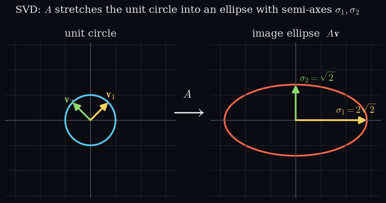
- SVD — factorises any matrix (square or not) into \(A = U\Sigma V^\top\): geometrically a rotation, then a stretch, then a rotation. Unlike diagonalization, it works for every matrix with no exceptions.
- The three pieces — \(U\) (left singular vectors) is orthonormal \(m\times m\); \(\Sigma\) has the singular values on its diagonal, same shape as \(A\), largest first; \(V\) (right singular vectors) is orthonormal \(n\times n\), and the equation uses \(V^\top\).
- The engine — singular values are the square roots of the eigenvalues of \(A^\top A\) (or \(AA^\top\); they share the same nonzero eigenvalues). For a \(2\times3\) matrix, \(AA^\top\) is only \(2\times2\), much smaller than the \(3\times3\) \(A^\top A\), so start there.
- Two valid routes — from \(AA^\top\) the eigenvectors give \(U\), then \(v_i = \tfrac{1}{\sigma_i}A^\top u_i\) gives \(V\); from \(A^\top A\) the eigenvectors give \(V\), then \(u_i = \tfrac{1}{\sigma_i}A v_i\) gives \(U\).
Two things people forget
Normalise every singular vector: SVD needs unit vectors, so divide each by its length. And transpose \(V\) at the end: the equation is \(U\Sigma V^\top\), not \(U\Sigma V\). Also, when \(A\) is wider than tall (like \(2\times3\)) the shortcut produces one fewer \(V\) column than needed, because the extra eigenvalue is \(0\) and you cannot divide by it. Fill the last column with the null space of \(A\) (the direction \(A\) crushes to zero), found by solving \(Av = 0\).
Step 1, singular values via \(AA^\top\)
Using the \(2\times2\) shortcut \(\lambda^2 - \operatorname{tr}\lambda + \det\), with trace \(34\) and determinant \(289 - 64 = 225\):
Eigenvalues \(25\) and \(9\), so the singular values are \(\sigma_1 = \sqrt{25} = 5\) and \(\sigma_2 = \sqrt{9} = 3\):
(\(\Sigma\) matches \(A\)'s shape; the extra zero column reflects that \(A\) is wider than tall.)
Step 2, \(U\) from the \(AA^\top\) eigenvectors
\(\lambda = 25\): \((AA^\top - 25I)u = 0\) gives \(u_1 = u_2\), so \((1,1)\) normalised is \(u_1 = \tfrac{1}{\sqrt2}(1,1)\). \(\lambda = 9\): gives \(u_1 = -u_2\), so \((1,-1)\) normalised is \(u_2 = \tfrac{1}{\sqrt2}(1,-1)\).
Step 3, \(v_1\) and \(v_2\) from the shortcut
Use \(v_i = \tfrac{1}{\sigma_i}A^\top u_i\):
Both come out unit length automatically.
Step 4, the third \(V\) column (null space)
\(V\) must be \(3\times3\), but the shortcut gave only two columns. The third is the direction \(A\) sends to zero, so solve \(Av = 0\):
Adding the equations gives \(v_1 = -v_2\); substituting gives \(v_2 = 2v_3\). Taking \(v_3 = 1\) yields \((-2, 2, 1)\), of length \(3\):
This is orthogonal to \(v_1\) and \(v_2\), and \(Av_3 = 0\) confirms it is the crushed direction.
Answer
The singular values \(5\) and \(3\) are the amounts \(A\) stretches along its two principal directions; the third \(V\) direction is collapsed to zero.
4.9 · SVD of a square matrix
Find the singular value decomposition of
Topics & Definitions
- Square still needs the transpose — even though \(A\) is square, SVD uses \(A^\top A\) (or \(AA^\top\)): the singular values are \(\sqrt{\text{eigenvalues of } A^\top A}\), never the eigenvalues of \(A\) itself.
- The matched-pair rule — which shortcut you use depends entirely on which matrix you started from. From \(A^\top A\) you get \(V\) first, then \(U\) via \(u_i = \tfrac{1}{\sigma_i}A v_i\) (plain \(A\)). From \(AA^\top\) you get \(U\) first, then \(V\) via \(v_i = \tfrac{1}{\sigma_i}A^\top u_i\) (transpose \(A^\top\)).
- The transpose follows the direction of travel — plain \(A\) moves you toward \(U\); transpose \(A^\top\) moves you toward \(V\). Memory hook: multiply what you have to produce what you want. Have \(V\), want \(U\): use \(A\). Have \(U\), want \(V\): use \(A^\top\). Exercise 4.8 started from \(AA^\top\) and used \(A^\top\); this one starts from \(A^\top A\), so it uses plain \(A\).
Two routes to the SVD, and how each finds \(U\) differently:
| Route 1, start from \(A^\top A\) | Route 2, start from \(AA^\top\) |
|---|---|
| Eigenvectors of \(A^\top A\) give you \(V\) directly | Eigenvectors of \(AA^\top\) give you \(U\) directly |
| Then find \(U\) with \(u_i = \tfrac{1}{\sigma_i}A v_i\) (plain \(A\)) | Then find \(V\) with \(v_i = \tfrac{1}{\sigma_i}A^\top u_i\) (transpose \(A^\top\)) |
The transpose is tied to the direction you travel, not to \(U\) or \(V\): plain \(A\) moves toward \(U\), transpose \(A^\top\) moves toward \(V\). This exercise used Route 1 (started from \(A^\top A\)), so \(U\) came from plain \(A\); exercise 4.8 used the opposite route, which is why it used \(A^\top\), same logic, different starting matrix.
Two easy slips
Normalise every vector (divide by its length), since SVD needs unit vectors. And when combining the singular-value fraction with the vector's own normalising fraction, simplify carefully: \(\tfrac{1}{2\sqrt2}\cdot\tfrac{1}{\sqrt2} = \tfrac14\) because \(\sqrt2\cdot\sqrt2 = 2\). Note \(2\sqrt2 = \sqrt8\), so \(\tfrac{1}{2\sqrt2}\) and \(\tfrac{1}{\sqrt8}\) are the same number.
Start from \(A^\top A\) (its eigenvectors are the \(V\) columns), read off the singular values, then travel to \(U\) with plain \(A\).
Step 1, singular values
Using \(\lambda^2 - \operatorname{tr}\lambda + \det\), with trace \(10\) and determinant \(25 - 9 = 16\):
Eigenvalues \(8\) and \(2\), so \(\sigma_1 = \sqrt8 = 2\sqrt2\) and \(\sigma_2 = \sqrt2\):
(Square \(A\) gives a square \(\Sigma\), no leftover zero column.)
Step 2, \(V\) from the \(A^\top A\) eigenvectors
Since we started from \(A^\top A\), its eigenvectors are the \(V\) columns. \(\lambda = 8\): \((A^\top A - 8I)v = 0\) gives \(v_1 = v_2\), so \((1,1)\) normalised is \(v_1 = \tfrac{1}{\sqrt2}(1, 1)\). \(\lambda = 2\): gives \(v_1 = -v_2\), so \((-1,1)\) normalised is \(v_2 = \tfrac{1}{\sqrt2}(-1, 1)\).
Step 3, \(U\) from the shortcut (plain \(A\))
We have \(V\) and want \(U\), so use \(u_i = \tfrac{1}{\sigma_i}A v_i\) with plain \(A\) (no transpose):
So \(U\) is the identity:
Answer
The singular values \(2\sqrt2\) and \(\sqrt2\) are the stretch amounts. Here \(U\) came out as the identity, so all the rotation lives in \(V^\top\). The lesson worth keeping: the choice between \(A\) and \(A^\top\) in the shortcut is dictated by which matrix you decomposed first, \(A^\top A\) gives \(V\) (then plain \(A\) for \(U\)), \(AA^\top\) gives \(U\) (then \(A^\top\) for \(V\)).
4.10 · Rank-1 approximation
Find the rank-1 approximation of
Topics & Definitions
- Rank-1 approximation — keep only the single strongest layer of the SVD: \(\hat A(1) = \sigma_1 u_1 v_1^\top\), using the largest singular value \(\sigma_1\), the first left-singular vector \(u_1\), and the first right-singular vector \(v_1\).
- Best possible (Eckart–Young) — this is the best rank-1 approximation of \(A\), and the approximation error is exactly \(\sigma_2\).
- Reuse the SVD — this reuses the SVD of \(A\) from Exercise 4.8, so no new decomposition is needed, just extract the "first" pieces.
- The outer product — \(u_1 v_1^\top\) is a column (\(m\times1\)) times a row (\(1\times n\)), producing a full \(m\times n\) matrix whose \((j,k)\) entry is \((u_1)_j (v_1)_k\).
Row vs column when reading \(V^\top\)
\(v_1\) is the first column of \(V\), which is the first row of \(V^\top\). Transposing swaps rows and columns, so when reading from \(V^\top\) take its rows to get the \(v_i\) vectors, not its columns. Reading down a column of \(V^\top\) by mistake mixes pieces of \(v_1, v_2, v_3\) together and gives wrong numbers.
Step 1, pull out the first pieces
From the SVD of \(A\) (Exercise 4.8):
\(\sigma_1\) is the largest singular value, \(u_1\) is the first column of \(U\), and \(v_1\) is the first row of \(V^\top\). Note the third entry of \(v_1\) is \(0\).
Step 2, outer product \(u_1 v_1^\top\)
Multiply the column by the row (each entry scaled by \(\tfrac{1}{\sqrt2}\cdot\tfrac{1}{\sqrt2} = \tfrac12\)):
Step 3, scale by \(\sigma_1\)
Answer
The two rows are identical because \(u_1 = \tfrac{1}{\sqrt2}(1,1)\) weights both output directions equally, and the third column is zero because \(v_1\) has a zero third entry. Compared with the original \(A = \begin{pmatrix}3&2&2\\2&3&-2\end{pmatrix}\), this rank-1 layer captures the dominant shared structure; the finer detail (the differences between entries and the \(-2\)) lives in the discarded \(\sigma_2\) layer, and the error it costs is exactly \(\sigma_2 = 3\).
4.11 · \(A^\top A\) and \(AA^\top\) share nonzero eigenvalues
Show that for any \(A \in \mathbb{R}^{m\times n}\), the matrices \(A^\top A\) and \(AA^\top\) have the same nonzero eigenvalues.
Topics & Definitions
- Why it matters — this justifies the SVD shortcut: since \(A^\top A\) and \(AA^\top\) share nonzero eigenvalues, the singular values \(\sqrt{\lambda}\) are the same whichever product you use, so you can diagonalize the smaller one.
- The key idea — if \(x\) is an eigenvector of \(A^\top A\), then \(Ax\) is an eigenvector of \(AA^\top\) with the same eigenvalue. Multiplying by \(A\) transfers the eigenvalue between the products; \(A\) itself is only the bridge.
- Why "nonzero" matters — the argument needs \(Ax \neq 0\) to give a genuine eigenvector, which is only guaranteed when \(\lambda \neq 0\).
Proof
Let \(\lambda \neq 0\) be an eigenvalue of \(A^\top A\) with eigenvector \(x \neq 0\):
Multiply on the left by \(A\):
Regroup using associativity:
This has the form of an eigenvalue equation for \(AA^\top\), with eigenvector \(Ax\) and eigenvalue \(\lambda\).
Check \(Ax \neq 0\): if \(Ax = 0\), then \(A^\top A\, x = A^\top(Ax) = 0 = \lambda x\), forcing \(\lambda = 0\) (since \(x \neq 0\)), contradicting \(\lambda \neq 0\). So \(Ax\) is a genuine eigenvector. The reverse direction is identical, swapping \(A\) and \(A^\top\) (start from \(AA^\top y = \lambda y\) and multiply by \(A^\top\)).
Conclusion
Every nonzero eigenvalue of \(A^\top A\) is a nonzero eigenvalue of \(AA^\top\), and vice versa, so the two matrices share exactly the same nonzero eigenvalues. \(\blacksquare\)
(They may differ in their zero eigenvalues: the larger matrix simply has extra zeros to fill its extra dimensions, which is why singular values come only from the nonzero eigenvalues.)
4.12 · The largest singular value is the maximum stretch
Show that for \(x \neq 0\),
where \(\sigma_1\) is the largest singular value of \(A \in \mathbb{R}^{m\times n}\).
Topics & Definitions
- The stretch factor — \(\lVert Ax\rVert / \lVert x\rVert\) measures how much \(A\) lengthens \(x\). This theorem says the most \(A\) can stretch any vector is exactly \(\sigma_1\), giving the largest singular value a concrete meaning: the matrix's maximum amplification.
- Orthogonal matrices preserve length — \(\lVert Uz\rVert = \lVert z\rVert\) and \(\lVert Vz\rVert = \lVert z\rVert\), which lets you strip \(U\) and \(V\) from \(A = U\Sigma V^\top\) and reduce the problem to the diagonal \(\Sigma\).
- \(\sigma_1\) is the largest — so every \(\sigma_i^2 \le \sigma_1^2\), which bounds the sum.
- Proving a maximum — needs two parts: an upper bound (nothing exceeds \(\sigma_1\)) and attainment (some vector reaches it).
Step 1, reduce to the diagonal matrix
Write \(A = U\Sigma V^\top\). For \(x \neq 0\), set \(y = V^\top x\); since \(V\) is orthogonal, \(\lVert y\rVert = \lVert x\rVert\). Using that \(U\) preserves length:
So \(\dfrac{\lVert Ax\rVert}{\lVert x\rVert} = \dfrac{\lVert \Sigma y\rVert}{\lVert y\rVert}\).
Step 2, upper bound
Since \(\Sigma\) is diagonal, \(\Sigma y = (\sigma_1 y_1, \sigma_2 y_2, \dots)\), so
(each \(\sigma_i^2\) replaced by the larger \(\sigma_1^2\)). Taking square roots:
Step 3, the bound is attained
Choose \(x = v_1\), the first right-singular vector. Then \(y = V^\top v_1 = e_1 = (1,0,\dots,0)\), so
Some vector reaches \(\sigma_1\), so the bound is tight.
Conclusion
The ratio is bounded above by \(\sigma_1\) for every \(x\) and equals \(\sigma_1\) when \(x = v_1\), so
The maximum stretch of \(A\) is its largest singular value, achieved along the first right-singular vector \(v_1\).
Spotted a mistake or a step that doesn't make sense? Open an issue and I'll fix it.
Finding these useful? A star on GitHub helps other learners find them.